Flows line, Chaos and Julia
Intro
The generalization of a system is simply illustrated as a set of equations that describe the evolution of the system, which might depend on a set of \(m\) equations involving one dimensional differential equations with \(n\) variables, which we shall call parameters of the system.
The simplest case involves a one dimensional non-time dependent system (i.e. autonomous system) of the form:
\begin{equation} \dot{x} = f(x) \end{equation}
where \(x\) is the state of the system and \(f(x)\) is a function of the state of the system.
However, the generalization of the system is not limited to this case, but it can be extended to a one dimensional time dependent system (i.e. nonautonomus system) with a simple coordinate transform.
As it might became non trivial to solve the system explicitly, we use a straightforward analytical method to study the dynamics of the system based on studying the behavior of the flow in the DE.
The Analytical Method
The analytical method is based on the following steps:
- Find the \(\dot{x} = f(x)\) function for your problem.
- Plot the function \(f(x)\).
- Note that the \(y\) axis corresponds to speeed, so if \(f(x) > 0\) the flow is going to the right, and if \(f(x) < 0\) the flow is going to the left. This will allow us to understand the behavior of the flow. To put it in other words, the flow is going to the right if \(f(x) > 0\) and to the left if \(f(x) < 0\).
- Note that some points will have \(f(x) = 0\), which means that the flow is not moving at all. This is called a fixed point.
- For each point, you can infer, if the flow at the left and the right are converging or diverging. This is called the stability of the fixed point. If the flow is converging, the fixed point is called stable (namely, sinks), and if the flow is diverging, the fixed point is called unstable (also known as sources).
Note how simple this method is, and how powerful it is. It allows us to understand the behavior of the system without solving the DE explicitly. Lets now tackle a simple example:
Example 1
Consider the following DE: \(\partial_t x= \cos{(x)}\)
- Just a toy example. Just write the DE in the form \(\dot{x} = \cos{(x)}\).
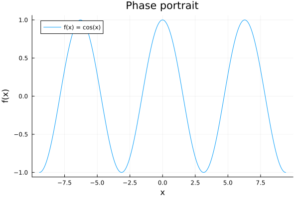
- Lets plot the phase portrait \(f(x) = \cos{(x)}\). This is called the Trajectory of the system.
f(x) = cos(x)
plot(f, -3π, 3π, label="f(x) = cos(x)")
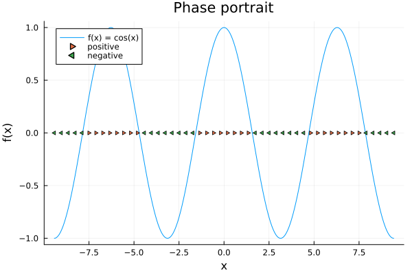
- Lets now plot the flow of the system…
Remember that if the function is positive, the flow is going to the right, and if the function is negative, the flow is going to the left. So, the flow is going to the right if \(\cos{(x)} > 0\) and to the left if \(\cos{(x)} < 0\).
xs = range(-3π, 3π, length=50)
ys = f.(xs)

# Keep only the positive values
positive_mask = ys .> 0
# Plot the positive values
scatter!(xs[positive_mask], ys[positive_mask].*0, label="positive", markershape=:rtriangle)

# Keep only the negative values
negative_mask = .!positive_mask
# Plot the negative values
scatter!(xs[negative_mask], ys[negative_mask].*0, label="negative", markershape=:ltriangle)
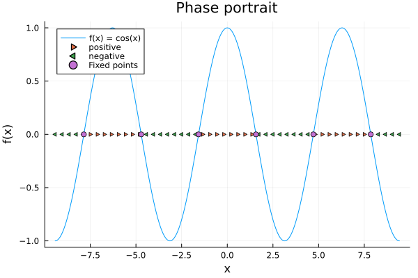
- Plot the fixed points of the flow. We remark that those correspond to equilibria of the system. In this case, we have infinite of them because the function is periodic.
# Scatter the points where the function is zero
interscet = Vector(-3π+0.5π :π:3π-.5π)
scatter!(interscet, f.(interscet), label="Fixed points", markershape=:circle)
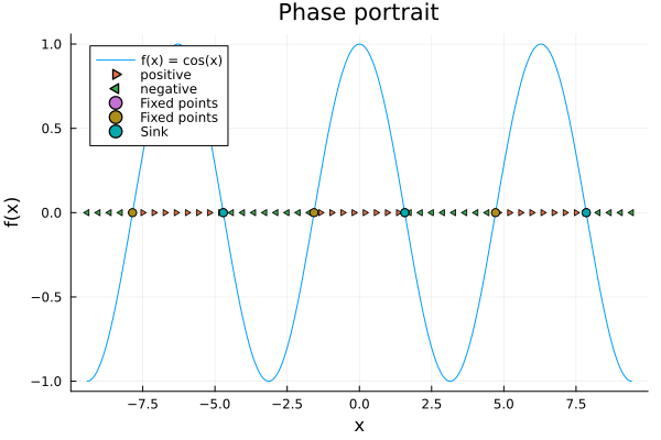
- Lets now study the stability of the fixed points. We remark that the flow is converging if the function is positive, and diverging if the function is negative. So, the flow is converging if \(\cos{(x)} > 0\) and diverging if \(\cos{(x)} < 0\).We’ll write a simple general function to do this.
function is_stalbe(x::Float64, f::Function; δ=0.1)
    # Check if the left goes up and the right goes to the left
    δ = abs(δ * x + 1e-10)
    if f(x-δ) > f(x) && f(x+δ) < f(x)
        return true
    end
    return false
end
Now, lets plot the stable and unstable fixed points.
stable = is_stalbe.(interscet, f)
scatter!(interscet[stable], f.(interscet[stable]), label="Sink", markershape=:circle)
Pretty simple, right? Lets now make some simulations to see how the system behaves in a real simulation.
function simulate(x0::Float64, f::Function; n::Int = 100, dt::Float64 = 0.1)
    x = x0
    xs = zeros(n)
    vs = zeros(n)
    for i in 1:n
        x += f(x) * dt
        @inbounds xs[i] = x
        @inbounds vs[i] = f(x)
    end
    return xs, vs
end;
Now that we can simulate a system, lets simulate the system for different initial conditions.
anim = @animate for x0 in rand(Vector(-2π:0.01:3π), 20)
    @fastmath simu_xs, simu_vs = simulate(x0, f)
    if simu_xs[1] > simu_xs[2]
        marks = :rtriangle
    else
        marks = :ltriangle
    end
    for t in eachindex(simu_xs)
        scatter(simu_xs[1:t], simu_vs[1:t], label=false, markershape=marks, xlabel="x", ylabel="f(x)", legend=:topleft, title="Phase portrait")
        plot!(f, -3π, 3π, label="f(x) = cos(x)")
    end
    scatter!([simu_xs[end]], [simu_vs[end]], label="Fixed points", markershape=:star4)
    scatter!([simu_xs[1]], [simu_vs[1]], label="Initial condition", markershape=:circle)
    sleep(0.5)
end
gif(anim, "flow.gif", fps = 1)
Do you notice something interesting in the simulation? Ofcourse!, It ends up in a fixed point, besides we start from a random initial condition. This is because the system is periodic, and it will always end up in the same fixed point. This is called a periodic orbit, but has no very important meaning in the 1D case. —
Linear stability
Besides the method above is very useful to understand the behavior of the system, it is not very useful to understand numerically the behavior of the system. For this, we need to use numerical methods. However, we can use the method above to understand the behavior of the system in the linear regime. This is called linearization.
The idea is to linearize the DE around a fixed point. This is done by using the Taylor expansion. The Taylor expansion is a method to approximate a function around a point. For example, if we want to approximate the function \(f(x)\) around the point \(x_0\), we can write:
\[f(x) = f(x_0) + f'(x_0)(x-x_0) + \frac{f''(x_0)}{2!}(x-x_0)^2 + \frac{f'''(x_0)}{3!}(x-x_0)^3 + \dots\]where \(f'(x_0)\) is the derivative of the function \(f(x)\) at the point \(x_0\), \(f''(x_0)\) is the second derivative of the function \(f(x)\) at the point \(x_0\), and so on.
The trick is to neglect all the terms that are not linear in \(x-x_0\). (i.e. the terms that are not linear in the perturbation).
WARNING: It is safe to to neglect the higher order terms if the function is smooth. If the function is not smooth (i.e, you can actually expand it) and if \(f'(x_0)\) is not zero, otherwise it would no longer be a leading order approximation.
In this manner, if we can rewrite the DE as: \(\dot{x} = f(x) = f(x_0) + f'(x_0)(x-x_0),\)
wich corresponds to the classic exponential growth or decay of a perturbation around a fixed point. Another important term arises here: the growth rate. The growth rate is the rate at which the perturbation grows or decays. In this case, the growth rate is given by \(f'(x_0)\).
The rate allow to define a characteristic time scale of the system at \(x_0\), which is the time it takes for the perturbation to grow or decay by a factor of \(e\). In this case, the characteristic time is given by \(1 / \|f'(x_0)\|\).
The stability at fixed points with inflection points is not generalizable to the linear regime, see for instance the example at these three examples. Let us first write a function to compute analytical solution for an abstract DE.
"""
analytic_solve: Analitically solve any one dimensional flow system
"""
function analytic_solve(f::Function, xs::AbstractArray; n::Int = 1000, δ::Float64=0.00001)
    # Plot the
    ys = f.(xs)
    plot(xs, ys, label="f(x)")
    # Plot the fixed points
    positive_mask = ys .> 0
    # Plot the positive values
    scatter!(xs[positive_mask], ys[positive_mask].*0, label="positive", markershape=:rtriangle)
    # Keep only the negative values
    negative_mask = .!positive_mask
    # Plot the negative values
    scatter!(xs[negative_mask], ys[negative_mask].*0, label="negative", markershape=:ltriangle)
    # Scatter the points where the function is zero
    closer_to_zero = abs.(f.(range(minimum(xs), maximum(xs), n))) .< δ
    interscet = range(minimum(xs), maximum(xs), n)[closer_to_zero]
    scatter!(interscet, f.(interscet), label="Fixed points", markershape=:circle)
    # Check if the fixed points are stable
    stable = is_stalbe.(interscet, f)
    scatter!(interscet[stable], f.(interscet[stable]), label="Sink", markershape=:circle)
end
Examples:
- \[\dot{x} = x^2\]
# Plot the function
xs = range(-3, 3, length=50)
f_1 = x -> x^2
analytic_solve(f_1, xs)
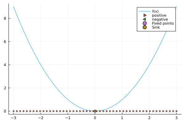 Do you see the problem? The function is not smooth, so we cannot expand it. And, when solving analytically, we see that it is a strange attractor from the left, and a repeller from the right. We call this a half-stable.
This is not general for all non-linearizable cases, as well see in the next two examples.
- \[\dot{x} = x^3\]
f_2 = x -> x^3
analytic_solve(f_2, xs)
In this case, we clearly see that the fixed point is a repeller.
- \[\dot{x} = -x^3\]
f_3 = x -> -x^3
analytic_solve(f_3, xs)
A simple sign change in the function, and we see that the fixed point is a sink and since we only have one fixed point, the system is globally stable.
Uniqueness
You might have noticed that we stated the analytic_solve as a universal solver… But it was a complete lie! The analytic solver works as expected if a solution is unique, which is given by the uniqueness theorem. The uniqueness theorem states that if the DE is autonomous, and if the DE has a unique solution, consider:
Then, the solution is unique and has solution in a interval \([x_0 - \delta x, x_0 + \delta x]\) if and only if the functions \(f(x)\) and \(f'(x)\) are continuous in a open interval \(\{x\} \in \mathbb{R}\)
Imposibility of occilations
Note that for a first order non-autonomous system, the system can either converge to a fixed point, or diverge to infinity. And it is very straight forward to see why, in the plots \(y=f(x)\) and \(y=\dot{x}\), the function (obviously) is singled valued, so it can no pass through the same point twice. This is called the imposibility of occilations.
From Flows to Potentials
In physics, we are more used to study systems in terms of potentials. The idea is to rewrite the DE in terms a potential \(V(x)\), which is a function that describes the energy of the system. The DE is then rewritten as:
\[\dot{x} = -\frac{\partial V(x)}{\partial x} \ \ \Rightarrow \ \ \frac{d x}{d t}= -\frac{\partial V(x)}{\partial x}\] \[V(x) = \int_{x_0}^x \dot{x} \ dx\]Note that the minus arises naturally to make the stable fixed points have a minimum of the potential, and the unstable fixed points have a maximum of the potential, but for both of them, equilibriums of the system. Notice also that \(V(t)\) is monotonically decreasing along trajectories.
Example:
Graph the potential of \(\dot{x} = x - x^3\), identify the fixed points and classify them as stable or unstable.
We can perform the integration (in this case, symbolic) to obtain the potential:
f_4(x) = x - x^3
@SymPy.syms x
V = SymPy.integrate(f_4(x), x)
plot(-V, -1.5, 1.5, label="V(x)")
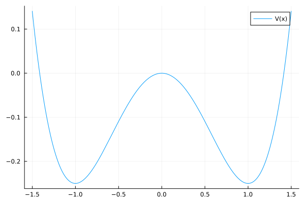
Therefore, we have three fixed points: \(x=0\), \(x=1\), and \(x=-1\), there is only one local maximum (corresponding to the source) at \(x=0\), and two local minimums (corresponding to the sinks) at \(x=1\) and \(x=-1\). This potential is called a double-well potential, and it is of special interest in particle physics, as it represents the Higgs potential… a one dimensional mexican hat.
Now, let’s use our analytic method to verify the results.
xs = range(-1.5, 1.5, length=50)
analytic_solve(f_4, xs; δ =0.01)
Summary
In this post, we have seen how to solve first order DEs, and how to use the analytic method to understand the behavior of the system. We have also seen how to linearize the DE around a fixed point, and how to use the growth rate to define a characteristic time scale of the system. Finally, we have seen how to rewrite the DE in terms of a potential, and how to identify the fixed points and classify them as stable or unstable.
Here are the main concepts:
- Vector Field: A vector field is a function that maps a point in space to a vector. In the case of DEs, the vector field is the function \(f(x)\), the plot corresponds to the phase portrait.
- Fixed Point: A fixed point is a point in space where the vector field is zero, corresponding to a equilibrium of the system.
- Stability: A fixed point is stable if the vector field points away from it, and unstable if the vector field points towards it.
- Global Stability: A fixed point is globally stable if all trajectories converge to it, and globally unstable if all trajectories diverge from it.
- Linearization: A linearization is a first order approximation of a function around a point. In the case of DEs, the linearization is a first order approximation of the vector field around a fixed point.
- Characteristic Time Scale: The characteristic time scale is the time it takes for a perturbation to grow or decay by a factor of \(e\). It is given by \(1/\|f'(x_0)\|\) where \(x_0\) is a fixed point.
- Potential: A potential is a function that describes the energy of the system. It is given by \(V(x) = \int_{x_0}^x \dot{x} \ dx\) where \(x_0\) is a fixed point.
Hope you enjoyed it! See you in the next post!
Reference: Nonlinear Dynamics and Chaos, by Steven Strogatz.