Phonons in a Body-Centered Cubic (BCC) lattice.
Phonons in a Body-Centered Cubic (BCC) lattice.
Introduction
A body-centered cubic (BCC) cell is one of the simplest and most common crystal structures found in solid-state materials. The BCC unit cell is characterized by a cubic lattice with lattice points at each corner and an additional lattice point at the center of the cube.
In a BCC lattice, each unit cell consists of lattice points (atoms) contributing to the total crystal structure. The BCC structure is found in many metallic elements, such as iron, chromium, and tungsten, due to its efficient packing and strong interatomic bonding. The study of phonons is crucial for understanding the behavior of crystal lattice vibrations, which are responsible for various physical properties, such as thermal conductivity and specific heat. The dispersion relation for phonons in a BCC cell describes the relationship between the phonon frequency and its wavevector, revealing how lattice vibrations propagate through the material.
Theoretical Background
The BCC lattice can be generated by the following primitive vectors:
\[\mathbf{a}_1 = \frac{a}{2}(\mathbf{\hat{x}} + \mathbf{\hat{y}} - \mathbf{\hat{z}}), \quad \mathbf{a}_2 = \frac{a}{2}(-\mathbf{\hat{x}} + \mathbf{\hat{y}} + \mathbf{\hat{z}}), \quad \mathbf{a}_3 = \frac{a}{2}(\mathbf{\hat{x}} - \mathbf{\hat{y}} + \mathbf{\hat{z}})\]Let’s begin by defining the position vectors for the two atoms in a BCC unit cell:
- \[\vec{R}_{1} = l\vec{a}_1 + m\vec{a}_2 + n\vec{a}_3\]
- \[\vec{R}_{2} = \left(l+\frac{1}{2}\right)\vec{a}_1 + \left(m+\frac{1}{2}\right)\vec{a}_2 + \left(n+\frac{1}{2}\right)\vec{a}_3\]
Now, let’s find the displacement vectors of the two atoms in the x-direction:
- \[u^x_{l,m,n} = u^x_1(l\vec{a}_1 + m\vec{a}_2 + n\vec{a}_3)\]
- \[u^x_{l+\frac{1}{2},m+\frac{1}{2},n+\frac{1}{2}} = u^x_2\left[\left(l+\frac{1}{2}\right)\vec{a}_1 + \left(m+\frac{1}{2}\right)\vec{a}_2 + \left(n+\frac{1}{2}\right)\vec{a}_3\right]\]
The potential energy of the system can be written as:
\[U = \frac{1}{2}C_1 \sum_{\langle i,j \rangle} \left(\vec{u}_i - \vec{u}_j\right)^2 + \frac{1}{2}C_2 \sum_{\langle\langle i,k \rangle\rangle} \left(\vec{u}_i - \vec{u}_k\right)^2\]where the first term represents the nearest neighbor interactions, and the second term represents the next-nearest neighbor interactions.
Using the displacements of the atoms, we can write the dynamical matrix \(D\) as:
\[D(\vec{k}) = \begin{bmatrix} \sum_{\vec{\delta}} C_1 \left(1 - e^{i\vec{k}\cdot\vec{\delta}}\right) + \sum_{\vec{\delta}'} C_2 \left(1 - e^{i\vec{k}\cdot\vec{\delta}'}\right) & -C_1 \left(1 - e^{i\vec{k}\cdot\vec{\delta}_{12}}\right) \\ -C_1 \left(1 - e^{i\vec{k}\cdot\vec{\delta}_{12}}\right) & \sum_{\vec{\delta}} C_1 \left(1 - e^{i\vec{k}\cdot\vec{\delta}}\right) + \sum_{\vec{\delta}'} C_2 \left(1 - e^{i\vec{k}\cdot\vec{\delta}'}\right) \end{bmatrix}\]Here, \(\vec{\delta}\) and \(\vec{\delta}'\) denote the position vectors of nearest neighbors and next-nearest neighbors, respectively, and \(\vec{\delta}_{12}\) is the position vector connecting atoms 1 and 2.
Now, solve the eigenvalue equation:
\[D(\vec{k})\vec{u} = \omega^2(\vec{k})\vec{u}\]where \(\omega(\vec{k})\) is the angular frequency of the normal modes, and \(\vec{u}\) is the eigenvector representing the mode. By solving this equation, we can find the dispersion relation \(\omega(\vec{k})\).
To find the eigenvalues, we’ll calculate the determinant of \((D(\vec{k}) - \omega^2(\vec{k})I)\) and set it equal to zero:
\[\text{det}\left(D(\vec{k}) - \omega^2(\vec{k})I\right) = 0\]This results in the following equation for the squared angular frequencies:
\[\left[\sum_{\vec{\delta}} C_1 \left(1 - e^{i\vec{k}\cdot\vec{\delta}}\right) + \sum_{\vec{\delta}'} C_2 \left(1 - e^{i\vec{k}\cdot\vec{\delta}'}\right) - \omega^2(\vec{k})\right]^2 - C_1^2 \left(1 - e^{i\vec{k}\cdot\vec{\delta}_{12}}\right)^2 = 0\]Solve this equation for \(\omega^2(\vec{k})\) to find the dispersion relation:
\[\omega^2(\vec{k}) = \sum_{\vec{\delta}} C_1 \left(1 - e^{i\vec{k}\cdot\vec{\delta}}\right) + \sum_{\vec{\delta}'} C_2 \left(1 - e^{i\vec{k}\cdot\vec{\delta}'}\right) \pm C_1 \left(1 - e^{i\vec{k}\cdot\vec{\delta}_{12}}\right)\]The \(\pm\) sign indicates that there are two branches in the dispersion relation for the phonon modes. To find the eigenvectors, we can substitute the obtained \(\omega^2(\vec{k})\) values back into the eigenvalue equation and solve for \(\vec{u}\). Using the dispersion relation we derived earlier:
\[\omega^2(\vec{k}) = \sum_{\vec{\delta}} C_1 \left(1 - e^{i\vec{k}\cdot\vec{\delta}}\right) + \sum_{\vec{\delta}'} C_2 \left(1 - e^{i\vec{k}\cdot\vec{\delta}'}\right) \pm C_1 \left(1 - e^{i\vec{k}\cdot\vec{\delta}_{12}}\right)\]Substituting this into the eigenvalue equation:
\[D(\vec{k})\vec{u} = \left[\sum_{\vec{\delta}} C_1 \left(1 - e^{i\vec{k}\cdot\vec{\delta}}\right) + \sum_{\vec{\delta}'} C_2 \left(1 - e^{i\vec{k}\cdot\vec{\delta}'}\right) \pm C_1 \left(1 - e^{i\vec{k}\cdot\vec{\delta}_{12}}\right)\right]\vec{u}\]Therefore we now know the eigenvalues of the dynamical matrix, which correspond to the squared angular frequencies of the phonon normal modes. To find the eigenvectors, we can substitute the eigenvalues back into the eigenvalue equation and solve for \(\vec{u}\).
To find the eigenvectors, we can substitute the eigenvalues back into the eigenvalue equation:
\[D(\vec{k})\vec{u} = \left[\sum_{\vec{\delta}} C_1 \left(1 - e^{i\vec{k}\cdot\vec{\delta}}\right) + \sum_{\vec{\delta}'} C_2 \left(1 - e^{i\vec{k}\cdot\vec{\delta}'}\right) \pm C_1 \left(1 - e^{i\vec{k}\cdot\vec{\delta}_{12}}\right)\right]\vec{u}\]Let’s rewrite the equation above as:
\[(D(\vec{k}) - \omega^2(\vec{k})I)\vec{u} = 0\]Now, we have a homogeneous system of linear equations, and we are looking for non-trivial solutions for the eigenvectors \(\vec{u}\). To do this, we can use any standard linear algebra method, such as Gaussian elimination, LU decomposition, or QR decomposition. Once we find the eigenvectors, they will represent the displacement of the atoms in the lattice for each phonon mode at a given wavevector \(\vec{k}\).
Then, we will use the eigenvectors to calculate the phonon dispersion relation (ofcourse by programming).
Lets code some stuff
using Plots

function phonon_dispersion(
    a = 1.0, # Lattice constant
    C1 = 1.0, # Spring constant
    C2 = 1.0, # Spring constant
)

    function ω²(q)
        # Compute the eigenstate for a given k vector
        C21 = C2/C1
        kx, ky, kz = q
        m11 = (2/3)*(-cos(0.5*(-kx*a+ky*a+kz*a))-cos(0.5*(kx*a+ky*a-kz*a))-cos(0.5*(kx*a-ky*a+kz*a))-cos(0.5*(kx*a+ky*a+kz*a))+4)-(2*C21*(cos(kx*a)-1))
        m12 = (2/3)*(cos(0.5*(-kx*a+ky*a+kz*a))-cos(0.5*(kx*a+ky*a-kz*a))+cos(0.5*(kx*a-ky*a+kz*a))-cos(0.5*(kx*a+ky*a+kz*a)))
        m13 = (2/3)*(cos(0.5*(-kx*a+ky*a+kz*a))+cos(0.5*(kx*a+ky*a-kz*a))-cos(0.5*(kx*a-ky*a+kz*a))-cos(0.5*(kx*a+ky*a+kz*a)))
        m22 = (2/3)*(-cos(0.5*(-kx*a+ky*a+kz*a))-cos(0.5*(kx*a+ky*a-kz*a))-cos(0.5*(kx*a-ky*a+kz*a))-cos(0.5*(kx*a+ky*a+kz*a))+4)-2*C21*(cos(ky*a)-1)
        m23 = (2/3)*(-cos(0.5*(-kx*a+ky*a+kz*a))+cos(0.5*(kx*a+ky*a-kz*a))+cos(0.5*(kx*a-ky*a+kz*a))-cos(0.5*(kx*a+ky*a+kz*a)))
        m33 = (2/3)*(-cos(0.5*(-kx*a+ky*a+kz*a))-cos(0.5*(kx*a+ky*a-kz*a))-cos(0.5*(kx*a-ky*a+kz*a))-cos(0.5*(kx*a+ky*a+kz*a))+4)-2*C21*(cos(kz*a)-1)
        matrix = [m11 m12 m13; m12 m22 m23; m13 m23 m33]
        values, eig = eigen(matrix)
        return values
    end

    Γ = [0, 0, 0]
    H = [0, 0, 2*pi/a]
    P = [pi/a, pi/a, pi/a]
    N = [0, pi/a, pi/a]

    points, labels = [Γ, H, P, Γ, N], ["Γ", "H", "P", "Γ", "N"]
    function bz_path(points, N)
        path = []
        for i in 1:(length(points) - 1)
            start_point = points[i]
            end_point = points[i + 1]
            for j in 0:N
                t = j / N
                q = start_point .+ t .* (end_point - start_point)
                push!(path, q)
            end
        end
        return path
    end

    N_points = 100
    path = bz_path(points, N_points)
    ωs² = [ω²(q) for q in path]
    ωs1² = [ωs²[i][1] for i in 1:length(ωs²)]
    ωs2² = [ωs²[i][2] for i in 1:length(ωs²)]
    ωs3² = [ωs²[i][3] for i in 1:length(ωs²)]
    plt = plot(
        ωs1²,
        label = "ω1²",
        xlabel = "q",
        ylabel = "ω²",
        title = "Phonon dispersion, C1 = $$C1, C2 = $$C2",
        xticks = (0:N_points:length(path), labels),
        legend = :topleft,
    )
    plot!(
        ωs2²,
        label = "ω2²",
    )
    plot!(
        ωs3²,
        label = "ω3²",
    )
end

phonon_dispersion(1.0, 10., 3.)
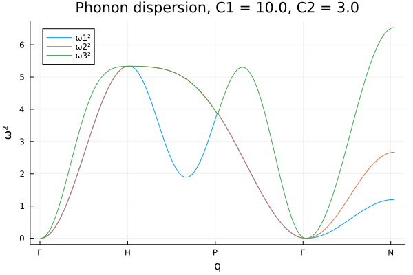
Note this result is in concordance with the result obtained in the reference http://lampz.tugraz.at/~hadley/ss1/phonons/bcc/bcc3.php. And now we can inspect the phonon dispersion relation for different values of the spring constants \(C_1\) and \(C_2\).
@gif for c2 = 0.1:0.2:40.
    for c1 = 0.1:0.2:20.
        phonon_dispersion(1.0, c1, c2)
    end
end