2D Orbits and bifurcations, Chaos and Julia
Intro
Some orbits present a periodic motion, that is, they repeat themselves after a certain time. These orbits are called closed orbits, but there is a very important characteristic regarding their neighborhood… If their near orbits are not closed, we call the trajectorie Isolated, and they only occur in non linear systems.
In this notebook we will see how to find the limit cycles of a dynamical system, and how to classify them.
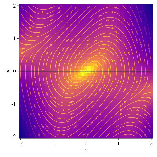
Example 1: Traditional Van der Pol oscillator: \(x'' + \mu(1-x^2)x' + x = 0\)
After rewriting the system in the form \(x' = f(x)\), we get:
\[\begin{cases} x' = y \\ y' = \mu(1-x^2)y - x \end{cases}\]μ = 1.
f11(x, y) = y
f12(x, y) = -x + μ*(1-x^2)*y
pde(x, y) = Point2f(f11(x, y), f12(x, y))
x = -2:0.1:2; y = -2:0.1:2
function plot_ode_makie(fx, fy, ode, x, y)
fig = CairoMakie.Figure(resolution = (600, 600), fontsize = 22, fonts = (;regular="CMU Serif"))
ax = fig[1, 1] = Axis(fig, xlabel = L"x", ylabel = L"y")
z = [log(f11(x, y)^2+f12(x, y)^2 ) for x in x, y in y]
fs = CairoMakie.heatmap!(ax, x, y, z, colormap = Reverse(:plasma))
CairoMakie.streamplot!(ax, pde, x, y, colormap = Reverse(:plasma), gridsize = (32, 32), arrow_size = 10)
CairoMakie.lines!(x, x.*0; color = :black, markersize = 10, label = "")
CairoMakie.lines!(x*0, x; color = :black, markersize = 10, label = "")
fig
end
plot_ode_makie(f11, f12, pde, x, y)
And we can also compute the numerical solution of the system:
function var_der_pol(du,u,p,t)
    x, y = u;  μ = p
    du[1] = y
    du[2] = -x .+ μ*(1-x^2)*y
end
u₀ = [0.5, 0.0]
tspan = (0.0, 20.0)
p = 1.5
prob = ODEProblem(var_der_pol,u₀,tspan,p)
sol = solve(prob);
Plots.plot([u[1] for u in sol.u], labels = "", lw = 3, xlabel = "t", ylabel = "x", title = "Van der Pol Oscillator")
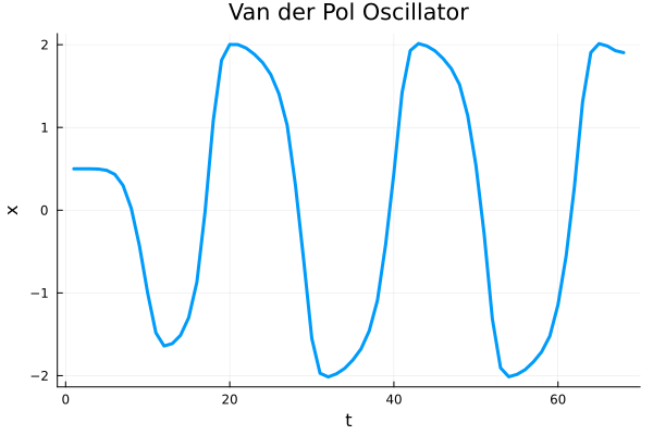
This is a very intereseting case because for \(\mu >> 1\) the system goes to what is called a strongly nonlinear regime. Oscillations are very small and are called relaxation oscillations, and the system is very sensitive to initial conditions.
μ = 10.
f12(x, y) = -x + μ*(1-x^2)*y
pde(x, y) = Point2f(f11(x, y), f12(x, y))
plot_ode_makie(f11, f12, pde, x, y)
Finding Limit Cycles
The interesting thing here is that the solution is periodic, but that is not always the same for general systems. There are a veriety of mathematical tools to find the limit cycles of a dynamical system, and to dig deeper I would recommend taking a deeper look at the book Dynamical Systems by Steven Strogatz. Some methods are:
- Gradient Systems: It deals with systems where \(\dot x = - \nabla V(x)\), where \(V(x)\) is a potential function. Here it is impossible to have closed orbits.
- Liapunov Functions: Lets take a system with \(\dot x = f(x)\), and define a function \(V(x)\) which is continuously differentiable and satisfies \(V(x) \geq 0\) and \(V(x^*) = 0\). Then, if \(V(x)\) is a Liapunov function, the system is stable if \(V'(x) \leq 0\) for all \(x\) in the neighborhood of the equilibrium point, and unstable if \(V'(x) \geq 0\) for all \(x\) in the neighborhood of the equilibrium point. If \(V'(x) = 0\) for all \(x\) in the neighborhood of the equilibrium point, then the system is neutral. Clearly, the big deal with this method is to find a function \(V(x)\) which is a Liapunov function.
- Dirac’s Method: If \(\dot x = f(x)\), and \(f(x)\) is continuously differentiable on a simply connected subset of the \((x, y)\) pĺane; and there exists \(g(x)\) s.t. one could construct \(\nabla\cdot (g f)\) and it doesn’t has a sign change, then there are no closed orbits.
And in order to demonstrate the contrary (there are closed orbits), we can use the following methods:
- Poincaré-Bendixson Theorem: If \(\dot x = f(x)\), and \(f(x)\) is continuously differentiable on a simply connected subset of the \((x, y)\) pĺane; and there exists a trajectory confined to a simply connected subset of the \((x, y)\) plane, then there are closed orbits.
The main reason why this theorem is so important is that it allows us to find the limit cycles of a dynamical system and thus it rules out the possibility of chaos in the 2D nonlinear case, but for higher dimensional cases, it no longer works.
Weekly nonlinear oscillations
In this section we sill see general equations of the form:
\[f(x) = \dot x = \epsilon h(x, \dot x) - x\]For any \(h(x, \dot x)\) smooth function. The idea is that when \(0<\epsilon \ll 1\) we get weakly nonlinear oscillations. It is very interesting to see that the general perturbation approach does not work here.
Let’s see this happening in the case of the damped harmonic oscillator:
\[\ddot x = -2 \epsilon \dot x - x\]Just to Recall, we have \(h(x, \dot x) = 2 \dot x\) Now, we can see that the solution by solving the system numerically:
function damped_occ(du, u, p, t)
    x, y = u;  ϵ = p
    du[1] = y
    du[2] = -2*ϵ*y - x
end
u₀ = [0., 1.]
tspan = (0.0, 50.0)
p = 0.1
prob = ODEProblem(damped_occ, u₀, tspan, p)
sol = solve(prob);
While solving it via the perturbation approach:
\(x(t) = \partial_t^2 (f) + 2 \epsilon \partial_t f + f = 0\) \((\ddot x_o + x_0) + \epsilon (\ddot + 2\dot x_- + x_1) + O(\epsilon^2) = 0\)
So after we put in the initial conditions, we get a linear combination of:
\[x_0 \approx \sin (t)\ \ \ \text{and} \ \ x_1(t) \approx -t sin(t)\]so it is:
\[x(t) = \sin(t) + \epsilon (-t \sin(t))\]Let us now compare the two solutions:
ϵ = 0.05
f_perturbation(t) = sin(t) - ϵ*t*sin(t)
ts = range(0, 50, length = 500)
xs_appr = [f_perturbation(t) for t in ts]
xs_real = [sol(t)[1] for t in ts]
@gif for i in 1:1:500
    p1 = Plots.plot(xs_real[1:i], labels = "Real Solution", lw = 3, xlabel = "t", ylabel = "x", title = "Damped Oscillator")
    Plots.plot!(xs_appr[1:i], label="Perturbation Th. Approximation", legend=:bottomleft)
    error = abs.(xs_real[1:i] .- xs_appr[1:i])
    p2 = Plots.plot(error, labels = "Error", lw = 3, xlabel = "t", ylabel = "x", title = "Residual", color=:red)
    Plots.plot(p1, p2, layout = (2, 1), size = (800, 600))
end
So clearly, the perturbation approach is quite descent until the first period, but afterwards, it starts having a serious error, this is a effect of our solution behaving slightly differently at two different time scales. One way of solving it is to do the perturbation a partial derivative at the two different time scales, but that is a bit more complicated and works well at scales of \(O(1/\epsilon)\).
Revisited bifurcations
Continuing with the 1D bifurcation theory, here we have a parameter that induces a topological change in the phase plane.
Saddle node bifurcations
This is the case when a pair or destruction of fixed points occurs. The normal case in 2D is given by:
\[\dot x = \mu - x^2\] \[\dot y = - y\]So clearly the decay rate in \(y\) happens at a fixed rate, while the bifurcation occurs in 1D for \(x\) axis at \(x^* =\pm \sqrt \mu\).
function plot_ode(fx, fy, xs, ys; to_scatter=[], title="", rescale=10)
    f(x, y) = log10((fx.(x, y).^2 + fy.(x, y).^2 +1))^0.5
    p1 = Plots.contour(xs, ys, f, xlims=(-2, 2), ylims=(-2, 2), colorbar = false, aspect_ratio = 1, legend = false, grid = false, framestyle = :zerolines, title = title)
    Plots.heatmap!(xs, ys, f, xlims=(-2, 2), ylims=(-2, 2))
    Plots.contour!(xs, ys, f, xlims=(-2, 2), ylims=(-2, 2), arrow_size = 0.1, color = :white)
    xs,ys = meshgrid(range(minimum(xs), stop=maximum(xs), length=20),
        range(minimum(ys), stop=maximum(ys), length=20))
    AAf(x, y) = [fx(x, y); fy(x, y) ] ./ (rescale*f(x, y))
    Plots.quiver!(xs, ys, quiver=AAf, c=:blue)
    if length(to_scatter) > 0
        Plots.scatter!([to_scatter[1][1]], [to_scatter[1][2]], color = :white, markersize = 10)
    end
    return p1
end

fy(x, y) = -y
xs = -2:0.1:2
ys = -2:0.1:2
@gif for μ = -2:0.1:2
    fx(x, y) = μ - (x^2)
    plot_ode(fx, fy, xs, ys; title = "Saddle Node Biffurcation, μ=$$μ")
end
Transcritical & Pitchfork
This extrapolation from 2D to 1D also applies for the other types of bifurcations we have seen, with a characteristic normal mode (for all, we take \(\dot y = -y\)):
- Transcritical: \(\dot x = \mu x - x^2\)
- Supercritical: \(\dot x = \mu x - x^3\)
- Subcritical: \(\dot x = \mu x + x^3\)
Example 2:
Let us proceed with the phase portrait of the system \(\dot x = \mu x - x^3\) for the three cases of \(\mu\):
function plot_supercriptical_pf(mu)
    f11_pc(x, y) = mu*x - x^3
    f12_pc(x, y) = -y
    plot_ode(f11_pc, f12_pc, xs, ys; title = "Supercritical Pithcfork, μ=$$mu", rescale = 20)
end
Thus, we note that:
- When \(\mu < 0\), there is only one fixed point at \(x^* = 0\), and the system is stable:
- At \(\mu = 0\), this shape remains but the key fact is that \(x\) decays with polynomial rate.
-
- At \(\mu > 0\), we have a saddle-node bifurcation, and we have two fixed points at \(x^* = \pm \sqrt \mu\).
@gif for μ in -2:0.1:2
    plot_supercriptical_pf(μ,)
end
It is also very interesting to see how the stability of the both fixed points changes in the transcritical case:
@gif for μ in -2:0.1:2
    f11_pc(x, y) = μ*x - x^2
    f12_pc(x, y) = -y
    plot_ode(f11_pc, f12_pc, xs, ys; title = "Transcritical Bifurcation, μ=$$μ", rescale = 20)
end
Hopf Bifurcation
The cases before all are consequence of having eigenvalues changing in the real part of the complex plane. Now, we will consider another case where the eigenvalues change in the imaginary part of the complex plane. This is the case of the Hopf bifurcation, and it is the case when a fixed point looses its stability.
Supercritical Hopf
Let’s suppose we have a damped oscillator whose damping is proportional to the tweakable parameter \(\mu\). There must be a critical value of \(\mu\) where the amplitude of the system starts increasing suddenly. A toy example for this is given by the system:
\[\dot r = \mu r - r^3\ \ \text{and} \ \ \dot \theta = \omega + br^2\]ω = 1.0; b = 1.
@gif for μ in -2:0.1:2
fx(x, y) = μ* x - ω*y
fy(x, y) = ω *x + μ*y
p1 = plot_ode(fx, fy, xs, ys; title = "Hopf Bifurcation, μ=$$μ", rescale = 10)
p2 = Plots.plot((x) -> 0, -2:0.1:2, colorbar = false, aspect_ratio = 1, legend = false, grid = false, framestyle = :zerolines, title="Eigenvalues")
Plots.scatter!([μ], [ω], label = "λ1", color = :red, xlabel="Re", ylabel="Im")
Plots.scatter!([μ], [-ω], label = "λ2", color = :blue)
Plots.plot(p1, p2, layout = (1, 2), size = (900, 600))
end
In general this happens in Hopfs bifurcations:
- The limit cycle grows proportionally to \(\sqrt{\mu-\mu_c}\).
- The limit is given by the \(\omega\) parameter.
Subcritical Hopf Bifurcation
In the same way a Pitchfork does, a subcritical change imposes a sudden jump in the state of the system. To see this, we can consider the following normal mode:
\[\dot r = \mu r + r^3 - r^5\ \ \text{and} \ \ \dot \theta = \omega + br^2\]Here the \(\mu\) makes the unsalability of the point tighten near the origin (inducted by the the \(r^3\) term), and the \(r^5\) term makes the limit cycle grow. This is like the catastrophe we saw before, as when the system starts oscillating and \(\mu>0\) we cannot stop it or return to the initial state.
ω = 0.5; b = 0.1
@gif for μ in -2:0.1:2
    fr(r, th) = μ*r + r^3 - r^5
    fth(r, th) = ω + b*r^2
    fx(x, y) = fr((x^2 + y^2)^0.5, atan(y, x)) * cos(atan(y, x)) - ((x^2+y^2)^0.5)*fth((x^2 + y^2)^0.5, atan(y, x)) * sin(atan(y, x))
    fy(x, y) = fr((x^2 + y^2)^0.5, atan(y, x)) * sin(atan(y, x)) + ((x^2+y^2)^0.5)*fth((x^2 + y^2)^0.5, atan(y, x)) * cos(atan(y, x))
    p1 = plot_ode(fx, fy, xs, ys; title = "Hopf Bifurcation, μ=$$μ", rescale = 50)
    p2 = Plots.plot((x) -> 0, -2:0.1:2, colorbar = false, aspect_ratio = 1, legend = false, grid = false, framestyle = :zerolines, title="Eigenvalues")
    Plots.scatter!([μ], [ω], label = "λ1", color = :red, xlabel="Re", ylabel="Im")
    Plots.scatter!([μ], [-ω], label = "λ2", color = :blue)
    Plots.plot(p1, p2, layout = (1, 2), size = (900, 600))
end
gif(anim, "hopf2_biff.gif", fps=10)
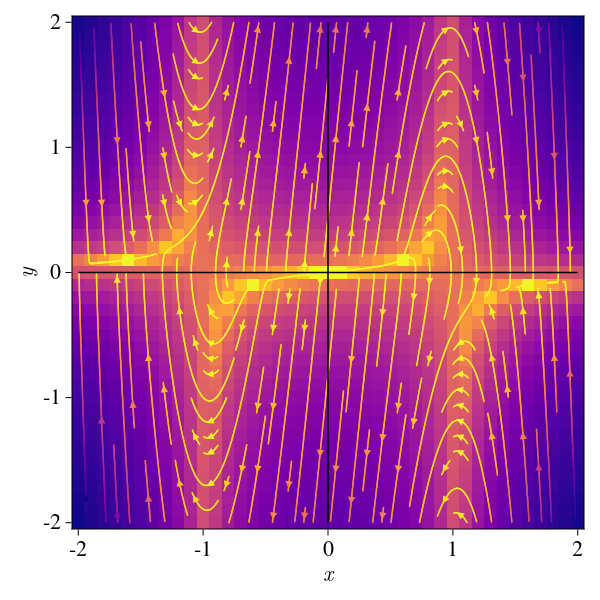
Example: As another example, we can consider the following system:
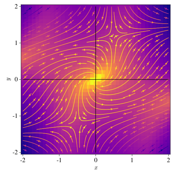
\[\dot x = \mu x-y+xy^2\ \ \text{and} \ \ \dot y = x + \mu y - y^3\]If we look at the Jacobian of this system, we get:
\[J = \begin{bmatrix} \mu - y^2 & -1 + 2xy \\ 1 & \mu - 3y^2 \end{bmatrix}\]And we note the system has it’s unique fixed point at \((0,0)\), so evaluating, the eigenvalues are:
\[\lambda_{1, 2} = \mu \pm i\]Which is a complex conjugate pair, so the system is unstable. Now, if we increase \(\mu\) we get to a positive value there arises a completelly unstable system:
μ = 1.0
fx(x, y) = μ *x - y + x*y^2
fy(x, y) = μ *y + x - y^3a
ode(x, y) = Point2f(fx(x, y), fy(x, y))
plot_ode_makie(fx, fy, ode, xs, ys)
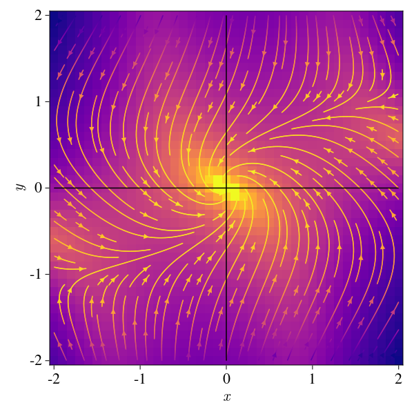
Whose critical point clearly appears at \(\mu < 0\), where we get stability near the origin.
μ = -1.
plot_ode_makie(fx, fy, ode, xs, ys)
Bifurcation of cycles
We have been seeing a lot how parameters induce change in the bahavior of fixed points. Now we will ask exactly the same question, but for cycles. The idea is that we will have a parameter that induces a change in the number of cycles of the system. This is the case of the Bifurcation of cycles, which can be achieved in 4 different mechanisms:
Saddle node bifurcation of cycles
As it happens with fixed points, we can have a saddle node bifurcation of cycles. This is the case when a pair of cycles are destroyed or created. The normal mode for this is given in the radial coordinates by the system:
\[\dot r= \mu r + r^3 - r^5\]The phenomenon is like a radial phase appears in the system at a fixed point \(\mu_c = -1/4\), as we’ll see:
fr(r,μ) = (r * μ + r^3 - r^5)
function plot_spiral(μ)
    xs = -2:0.1:2; ys = -2:0.1:2
    fr(r, th) = μ*r + r^3 - r^5
    fth(r, th) = ω + b*r^2
    fx(x, y) = fr((x^2 + y^2)^0.5, atan(y, x)) * cos(atan(y, x)) - ((x^2+y^2)^0.5)*fth((x^2 + y^2)^0.5, atan(y, x)) * sin(atan(y, x))
    fy(x, y) = fr((x^2 + y^2)^0.5, atan(y, x)) * sin(atan(y, x)) + ((x^2+y^2)^0.5)*fth((x^2 + y^2)^0.5, atan(y, x)) * cos(atan(y, x))
    f(x, y) = log10((fx.(x, y).^2 + fy.(x, y).^2 +1))^0.5
    p1 = Plots.contour(xs, ys, f, xlims=(-2, 2), ylims=(-2, 2), colorbar = false, aspect_ratio = 1, legend = false, grid = false, framestyle = :zerolines, title = "μ=$$μ")
    Plots.heatmap!(xs, ys, f, xlims=(-2, 2), ylims=(-2, 2))
    Plots.contour!(xs, ys, f, xlims=(-2, 2), ylims=(-2, 2), arrow_size = 0.1, color = :white)
    xs,ys = meshgrid(range(minimum(xs), stop=maximum(xs), length=20), range(minimum(ys), stop=maximum(ys), length=20))
    AAf(x, y) = [fx(x, y); fy(x, y) ] ./ (50*f(x, y))
    Plots.quiver!(xs, ys, quiver=AAf, c=:blue)
    return p1
end
function plot_r_axis(rs, μ)
    ys = fr.(rs, μ)
    Plots.plot(rs, ys, colorbar = false, aspect_ratio = 1, legend = false, grid = false, framestyle = :zerolines, title="Spiral")
end
@gif for μ in -1:0.01:-0.
    p1 = plot_spiral(μ)
    p2 = plot_r_axis(0:0.1:1, μ)
    Plots.plot(p1, p2, layout = (1, 2), size = (900, 600))
end
A very similar phenomenon happens when the convergence to a point happens on the case when the limit cycle approaches to the saddle point, which is called: Homoclinic Bifurcation, or one that that doesn’t allow for a limit cycle, which is called Infinite Period Bifurcation.
Conclusions
In this entry, we saw how a 2D nonlinear can be studied quite simply via the usage of the cycle limits and their regime… We also saw that the bifurcations can be studied in 1D, and that the bifurcations of cycles are quite similar to the bifurcations of fixed points in the 2D case, which can, in principle be studied on the line projection.
Hope you enjoyed it! See you in the next post!
Reference: Nonlinear Dynamics and Chaos, by Steven Strogatz.