The Lorenz Attractor, Chaos and Julia
Intro
Now we have arrived to the point where all modern chaos theory started from. For now lets treat them as mere black boxes and see what they do. We call the system, the Lorenz system:
\[\dot x = \sigma(y-x)\] \[\dot y = rx -y -xs\] \[\dot z = xy - bz\]where \(\sigma\), \(r\) and \(b\) are constants. The system is defined on the state space \(\mathbb{R}^3\), which was initially supposed to be a description of the dynamics of the atmpsphere. The system is nonlinear and deterministic. The system is chaotic if the initial conditions are close enough to each other. The system is sensitive to initial conditions. The system is periodic if the initial conditions are far enough from each other. The system is sensitive to parameters. The system is sensitive to initial conditions and parameters.
The key insight Lorentz had was noticing that the trajectory was always in a specific region of the space, but it was neither a fixed point or a closed trajectory, but a fractal.
Chaotic waterwheel
The main idea of this experiment created at MIT in the 70s is to simulate a system very similar to the one Lorentz initially had with. The idea is to have a constant water flow which is being pumped into a system of a several buckets. The thing, as shown in the following real experiment is that the final speed of the wheel highly depends on the initial configuration in the system.

If one were to actually do the math we would have to integrate all the mass contained between two angles, and the torque and angular acceleration associated with that mass. All the computation is a bit too much for this notebook, but the idea is that the system is described by the following equations:
\[\dot a_1 = \omega b_1 - K a_1\] \[\dot b_1 = -\omega a_1 - K b_1 + q_1\] \[\dot \omega = \frac{1}{I} \left(\pi g r a_1 - \omega v \right)\]Here, the coefficients \(a_n\), \(b_n\) are the amplitudes of the Fourier analysis of the variable \(m(\theta, t)\), \(q_n\) the coefficients of the decomposition of the water inflow \(Q(\theta)\), and \(I\) the moment of inertia of the wheel.
If we focus for now in finding the fixed points, and we set all derivatives to zero, we get various fixed points, which are the following:
\[(\omega = 0, a_1 =0, b_1 = q_1/K)\] \[(\omega = \sqrt{\pm \pi g r q_1/v - K^2}, b_1 = K v /\pi g r, a_1 = \omega K v /\pi g r K)\]So, we basically got a set of equations the pretty much follow the dynamics of the original Lorentz one.
Simple properties
The system, in Lorenzian form is:
\[\dot x = \sigma(y-x)\] \[\dot y = rx -y -xs\] \[\dot z = xy - bz\]where \(\sigma\) (Prandtl number), \(r\) (Rayleight number). As we can see, there are mainly two things which are making the system be nonlinear, the crossed products \(xy\) and \(xz\). The set is also time symmetric, and it has a quality named dissipative, meaning that the surface it spans is always contracting.
With respect to the fixed points, by looking at the extrema of the coordinates, we find two types of fixed points:
\[(x = 0, y = 0, z = 0)\] \[(x = y = \pm \sqrt{b(r-1)}, z = r - 1)\]Just to study the overall behavior, a linearization yields that the origin is kind of a saddle point, but the 3D shape makes it have one direction in and two out.
Moreover, if \(r < 1\) the system is globally stable (callback to it having all trajectories in \(\mathbb{R}^3\) converging to it and being Liapunov). If \(r > 1\) the system is unstable, and that’s where the fun begins.
The Lorenz attractor
Lets take back a minute the case where \(r > 1\). We see in the non-center fixed point that there are two possible paths, having both \(x, y\) positives (what Lorentz called \(C^+\)) or negatives \(C^-\). In the middle of them, we have to have a Hopf bifurcation, which is in fat given by the critical point:
\[r_H = \frac{\sigma(\sigma + b + 3)}{\sigma - b -1}\]Lorenz started with a point at \(\sigma=10\), \(r=28\), \(b=8/3\). The critical point is \(r_H = 24.74\), and studied how the coordinates behave:
function p_lorenz!(du, u, p, t)
    x, y, z = u      #variables are part of vector array u
    σ, ρ, β, = p     #coefficients are part of vector array p
    du[1] = dx = σ*(y-x)
    du[2] = dy = x*(ρ-z) - y
    du[3] = dz = x*y - β*z
end
#Initial conditions. x=1.0, y=0.0, z=0.0
u0 = [0., 1., 0.]
#Timespan of the simulation. 100 in this case.
tspan = (0.0, 1000.0)
#Coefficients of the functions.
p = [10.0, 28.0, 8/3]
#Feeding the inputs to the solver
prob = ODEProblem(p_lorenz!, u0, tspan, p)
sol = solve(prob);
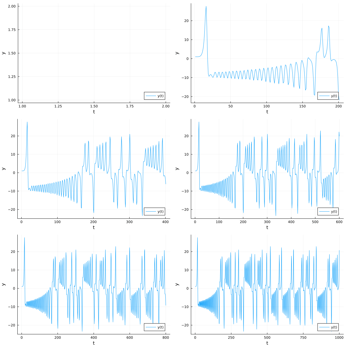
If we plot only the evolution of the \(x\) coordinate, we get a totally acyclic one:
@gif for i in 1:1000
    Plots.plot([1:i], [s[2] for s in sol.u[1:i]], ylabel="y", xlabel="t", label="y(t)", legend=:bottomright)
end

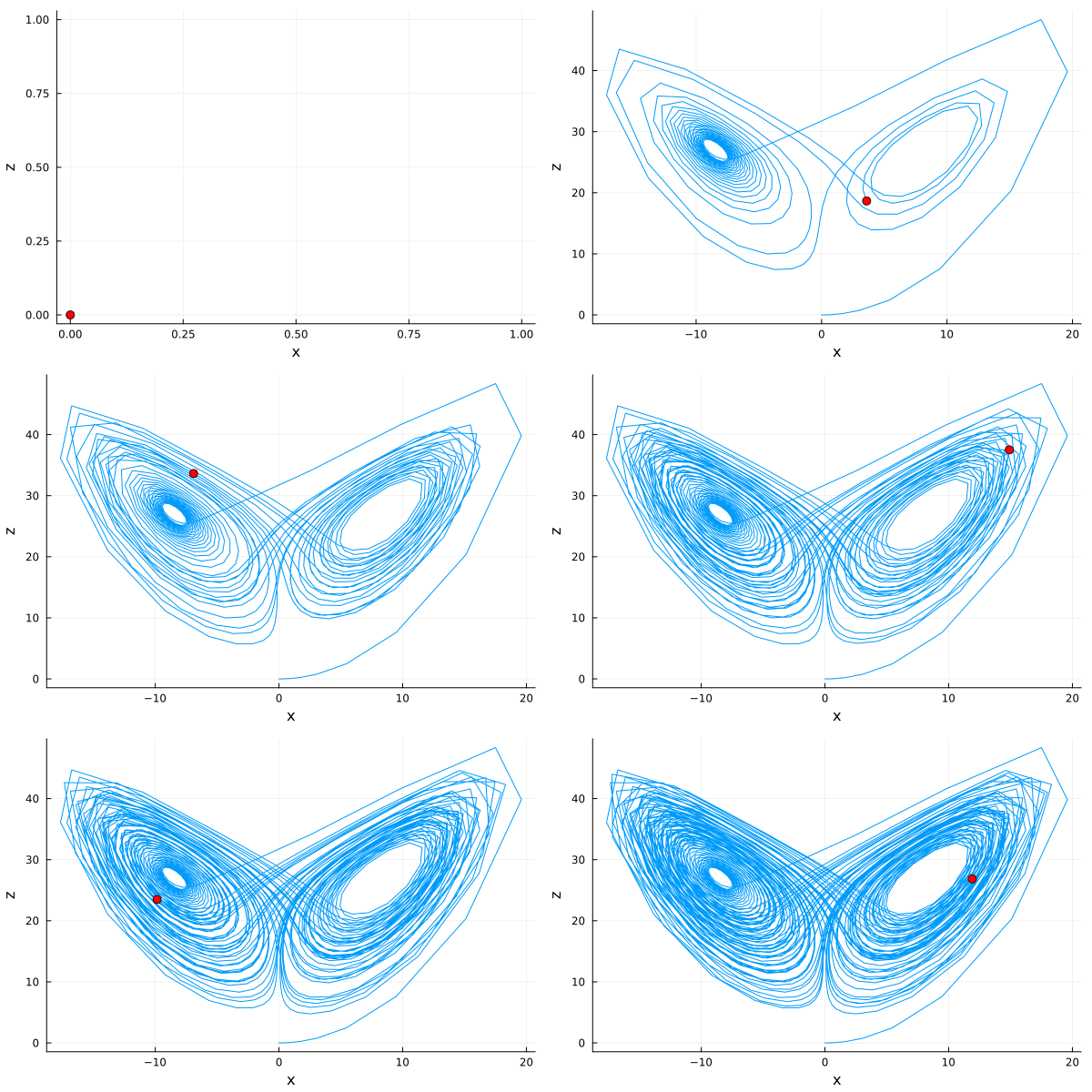
And there is a very complex behavior when we look at the plane \(x, z\):
ts = 0:0.05:100
sol = solve(prob, Tsit5(), saveat=ts);
@gif for i in 1:Integer(100/0.05)
    Plots.plot([s[1] for s in sol.u[1:i]], [s[3] for s in sol.u[1:i]], ylabel="z", xlabel="x", label="")
    Plots.scatter!([sol.u[i][1]], [sol.u[i][3]], label="", color=:red, markersize=5)
end

Besides it looks like trayectories do intersect, they don’t… It is just a projection of the 3D space. The 3D space is a fractal, and it is called the Lorenz attractor, which is a set of points with zero volume, but infinite surface.
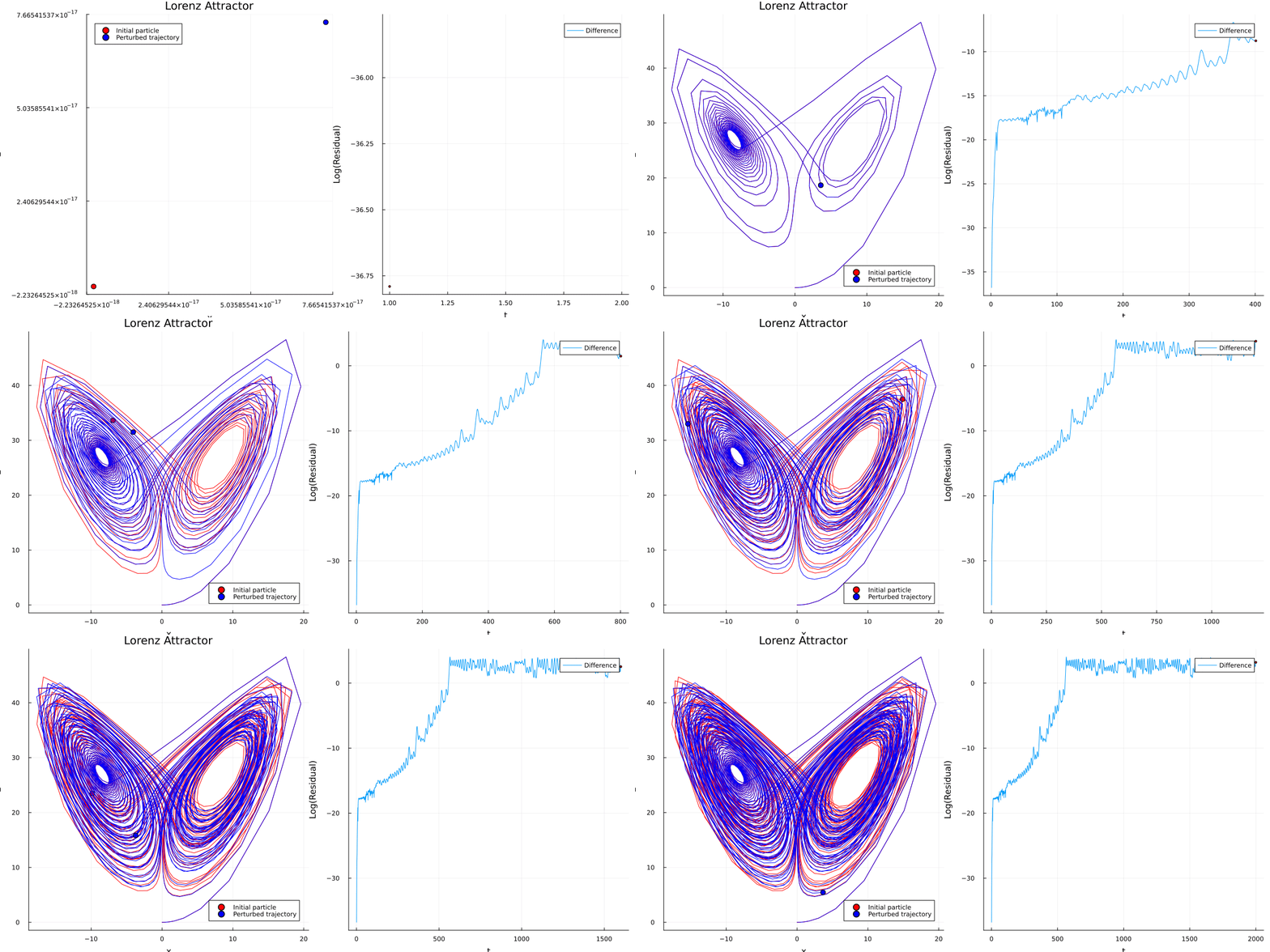
All the chaos get’s manifested when we look at the evolution of the \(x, y, z\) coordinates for slightly different initial conditions, creating a rapid divergence between trajectories, so that the uncertainty in the initial conditions is amplified by the system. This is called sensitivity to initial conditions.
For instance, lets suppose two trajectories start with a slight percentage difference of only \(\| \delta_0 \| \approx 10^{-15}\). For those trajectories, the difference in the paths is a function of time:
\[\| \delta \| \sim \| \delta_0 \| e^{t/\tau}\]where \(\tau\) is the Lyapunov time. The Lyapunov time is the time it takes for the trajectories to diverge by a factor of \(e\). The Lyapunov time is a measure of the sensitivity of the system to initial conditions. This difference should grow exponentially, but it will reach a maximum, which is obviously the total diameter of the attractor.
In fact, we can show this in a very simple experiment:
# We will deviate both trajectories by this amount
δ_0 = 1e-15

u_1 = [0., 1., 0.]
u_d = u_1 .+ rand().*δ_0

# Solving both systems....
prob_1 = ODEProblem(p_lorenz!, u_1, tspan, p)
prob_d = ODEProblem(p_lorenz!, u_d, tspan, p)
sol_1 = solve(prob_1, Tsit5(), saveat=ts);
sol_d = solve(prob_d, Tsit5(), saveat=ts);
Let us now plot the difference between the two trajectories:
differences = [norm(sol_1.u[i] - sol_d.u[i]) for i in 1:length(sol_1.u)]
@gif for i in 1:Integer(100/0.05)
    p1 = Plots.plot([s[1] for s in sol_1.u[1:i]], [s[2] for s in sol_1.u[1:i]], [s[3] for s in sol_1.u[1:i]], ylabel="y", xlabel="x", zlabel="z", label="", color=:red)
    Plots.scatter!([sol_1.u[i][1]], [sol_1.u[i][3]], label="Initial particle", color=:red, markersize=5, title = "Lorenz Attractor")
    Plots.plot!([s[1] for s in sol_d.u[1:i]],[s[2] for s in sol_1.u[1:i]], [s[3] for s in sol_d.u[1:i]], label="", color=:blue)
    Plots.scatter!([sol_d.u[i][1]], [sol_d.u[i][3]], label="Perturbed trajectory", color=:blue, markersize=5)
    difference = norm(sol_1.u[i] - sol_d.u[i])
    p2 = Plots.plot([1:i], log.([differences[j] for j in 1:i]), ylabel="Log(Residual)", xlabel="t", label="Difference", legend=:topright)
    Plots.scatter!([i], [log(difference)], label="", color=:red, markersize=2)
    Plots.plot!(p1, p2, layout=(1,2), size=(1200, 600))
end

This tool is a great way of estimating, up to a tolerance of \(a\), who many steps in the future it is going to be possible to have a valuable prediction, given by the maximum initial uncertainty of \(\| \delta_0 \|\). It is given by:
\[\tau = O\Big( \ln(\frac{a}{\| \delta_0 \|})^{1/\lambda} \Big)\]Generating definitions
As we can see, there are a lot of definitions, however not all of them are generally global. This first appearance of the Lorenz system allow us to dfine:
- Atractor: A set of the phase plane to which all trajectories converge at some point. If it is a normal one, the difference for trajectories starting at different points is bounded and goes to \(0\) as \(t \to \infty\). Moreover, an attartctor si a minimal set, so can we cannot have an attractor inside another one.
- Strange attractor: We define it as a type of attractor which is simply highly sensitive to the initial conditions.
The Lorenz map
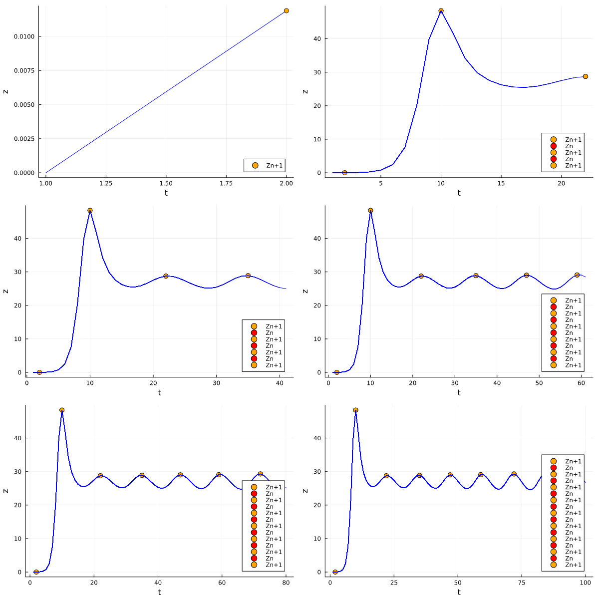
Lorenz noticed that it is in theory possible to focus on the \(z_n\) local maximum of the system, rather than the whole attractor. So one would try to predict which is going to be the next maximum and its time, given the current one. Here we are going to illustrate this idea:
next_found = false
Plots.plot()
@gif for i in 2:100
    global next_found
    Plots.plot!([1:i], [s[3] for s in sol.u[1:i]], ylabel="z", xlabel="t", label="y(t)", legend=:bottomright, label="", color=:blue)
    # Is a maximum?
    if sol[i][3] > sol[i-1][3] && sol[i][3] > sol[i+1][3]
        Plots.scatter!([i], [sol[i][3]], label="Zn", color=:red, markersize=5)
        next_found = false
    end
    if !next_found
        for f in eachindex(sol.u[i+1:end-1])
            k = i + f
            if sol.u[k][3] > sol.u[k-1][3] && sol.u[k][3] > sol.u[k+1][3] && !next_found
                next_found = true
                Plots.scatter!([i], [sol[i][3]], label="Zn+1", color=:orange, markersize=5)
            end
        end
    end
end

We will further inspect the Lorenz system, and we will see that it is possible to reduce it to a 1D map. But that is the topic of the next post… So, hope you enjoyed it! See you in the next post!
Reference: Nonlinear Dynamics and Chaos, by Steven Strogatz.